
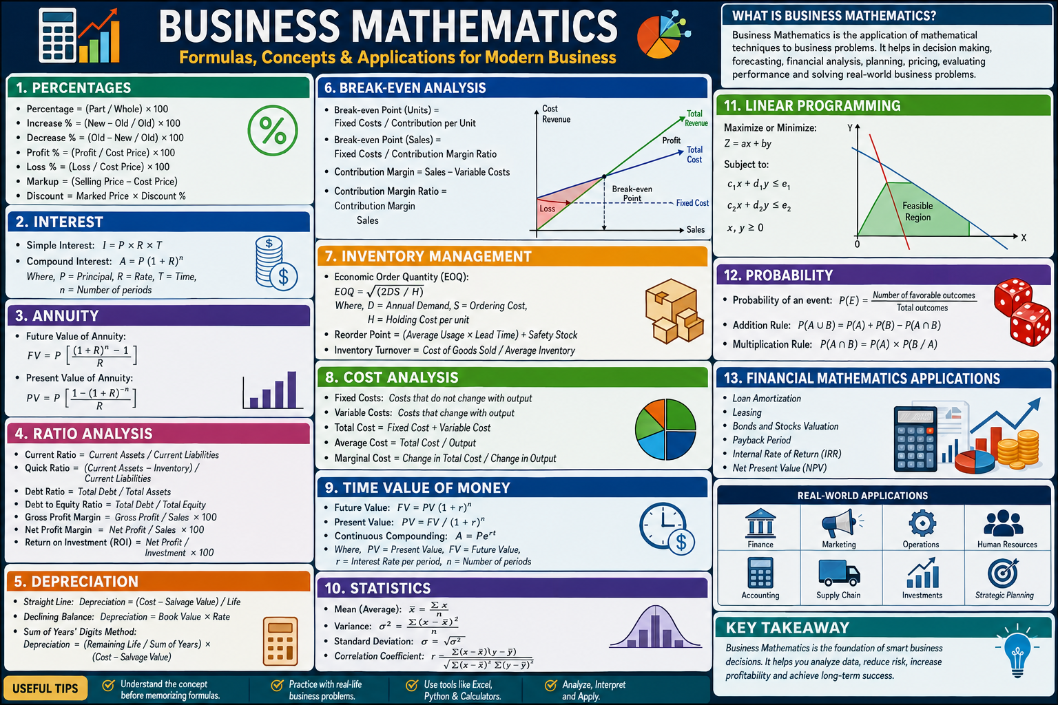
A Modern Tutorial Guide to Quantitative Reasoning in Commerce, Finance, and Strategy
Introduction
Why Business Mathematics Still Matters
Every commercial decision, however intuitive it may feel in the moment, ultimately rests on a quantitative skeleton. When a retailer sets a price, a bank prices a loan, a factory decides how many units to produce, or a board evaluates a merger, the reasoning underneath the decision is mathematical. Business mathematics is the discipline that formalises this reasoning — the arithmetic of percentages and interest, the algebra of break-even points, the linear systems behind resource allocation, and the statistics behind forecasting demand.
This document treats business mathematics as an anatomy: a body of interconnected structures, each performing a distinct function, together forming a working organism. Just as a physician studies bones, muscles, and organs separately before understanding how they cooperate, this guide separates business mathematics into its constituent ‘organs’ — interest theory, cost structures, matrix systems, optimisation, and statistical inference — before showing how modern practitioners assemble them into working financial models using spreadsheets and code.
The guide is deliberately dual in character. The first half builds the classical skeleton: the formulas and relationships that have underpinned commercial arithmetic for over a century. The second half is a ‘modern tutorial’ layer, showing how the same relationships are implemented today in spreadsheets, Python, and simple decision-support tools — because the mathematics has not changed, but the instruments used to apply it have.
It is worth stating plainly why this subject rewards careful study rather than superficial familiarity. Many of the errors that damage real businesses — mispricing a product, misjudging a break-even volume, underestimating the interest cost of a loan, or misreading a variance report — are not failures of judgement in the abstract; they are failures to apply a well-known formula correctly, or to notice which formula the situation actually calls for. A manager who can distinguish markup from margin, or a price variance from a volume variance, makes measurably better decisions than one who cannot, even holding all other business acumen constant. Mathematical fluency is, in this sense, a form of risk management in its own right.
How to use this document
Each chapter follows the same rhythm: the underlying concept, the core formula, a worked numerical example, and a short ‘modern application’ note showing how the same calculation is done with software. Readers may work through the document sequentially as a course, or use individual chapters as standalone reference sheets.Copy Section
Chapter 1
The Foundations — Ratios, Proportions, and Percentages
Percentages are the connective tissue of business mathematics. A percentage is simply a ratio expressed relative to 100, and almost every higher structure in this guide — interest rates, margins, growth rates, tax rates — is a percentage relationship in disguise.
A ratio compares two quantities of the same kind (for example, current assets to current liabilities), while a proportion asserts that two ratios are equal. Businesses use proportional reasoning constantly: scaling a recipe of raw materials for a larger production run, adjusting a marketing budget in proportion to expected revenue, or apportioning shared costs between departments according to headcount.
The percentage change formula, (New Value − Old Value) / Old Value × 100, is arguably the single most-used equation in commercial reporting. It underlies revenue growth statistics, inflation adjustments, year-on-year comparisons, and key performance indicator dashboards. A closely related idea is the percentage point, which measures an absolute change in a percentage figure rather than a relative change — a distinction routinely confused in financial journalism but critical in precise reporting (an interest rate moving from 5% to 7% is a two percentage point rise, but a 40% relative increase).
Worked Example — Percentage Change
A company’s quarterly revenue rises from R2,400,000 to R2,760,000. Percentage change = (2,760,000 − 2,400,000) / 2,400,000 × 100 = 15%. If the target growth rate was 12%, the company exceeded target by 3 percentage points, not ‘3% more’ — a distinction that matters when reporting to a board.
Modern ApplicationIn spreadsheets, percentage change is typically written as =(B2-A2)/A2 formatted as a percentage. In Python, growth = (new – old) / old, often vectorised across a pandas Series with .pct_change().Copy Section
Chapter 2
Index Numbers and Weighted Averages
Beyond a single percentage, businesses frequently need to track a composite measure built from many components — a basket of input costs, a portfolio of products, or a set of regional sales figures with different sizes of importance. Index numbers and weighted averages provide the mathematical structure for this aggregation.
An index number expresses a value in a given period relative to a fixed base period, conventionally set at 100. A simple price index is Index = (Current Price / Base Price) × 100; a weighted index, such as those used to construct inflation measures or input-cost trackers, applies a weight to each component reflecting its relative importance: Weighted Index = Σ(wᵢ × Iᵢ) / Σwᵢ, where wᵢ is the weight and Iᵢ is the individual index value of component i.
The weighted average is the same idea applied to raw values rather than index numbers, and is indispensable wherever simple averaging would mislead — for example, computing an average selling price across products with very different sales volumes, or an average cost of capital across debt and equity components weighted by their proportion of total financing (the weighted average cost of capital, or WACC, used throughout corporate finance).
Worked Example — Weighted Average Cost of Capital
A firm is financed 60% by equity (cost 14%) and 40% by debt (after-tax cost 7%). WACC = (0.60 × 14%) + (0.40 × 7%) = 8.4% + 2.8% = 11.2%. This blended rate, not either individual cost, is the correct discount rate for evaluating the firm’s average investment project.
Modern ApplicationWeighted averages are computed in spreadsheets with SUMPRODUCT(weights, values)/SUM(weights), and in Python with numpy.average(values, weights=weights) — both avoiding the error of simply averaging the raw figures unweighted.Copy Section
Chapter 3
Simple and Compound Interest
Interest is the price of money over time, and business mathematics distinguishes sharply between simple and compound interest because the distinction compounds — quite literally — into enormous differences over long horizons.
Simple interest accrues only on the original principal: I = P × r × t, where P is principal, r is the annual rate, and t is time in years. It is used for short-term instruments such as treasury bills and some consumer loans.
Compound interest accrues on both principal and previously earned interest, producing the exponential growth curve that underlies almost all long-term saving, investment, and debt calculations: A = P(1 + r/n)^(nt), where n is the number of compounding periods per year. The more frequently interest compounds — annually, monthly, daily, or continuously — the faster the balance grows for a given nominal rate, which is why lenders quote an effective annual rate (EAR) alongside a nominal rate to allow fair comparison across compounding frequencies.
The effective annual rate is calculated as EAR = (1 + r/n)^n − 1, and is the figure that should always be used when comparing two credit or savings products quoted with different compounding conventions — a 12% rate compounded monthly (EAR ≈ 12.68%) is genuinely more expensive than a 12.5% rate compounded annually (EAR = 12.5%), a comparison that the nominal rates alone would get backwards.
Worked Example — Compound Growth
R50,000 invested at a nominal annual rate of 9%, compounded monthly, for 10 years: A = 50,000 × (1 + 0.09/12)^(12×10) ≈ R122,894. The same principal under simple interest over the same period would grow to only R95,000 — a difference of almost R28,000 purely from the mechanics of compounding.
Modern ApplicationExcel and Google Sheets provide =FV(rate, nper, pmt, pv) to compute future value directly. In Python, the same calculation is A = P * (1 + r/n)**(n*t), and libraries such as numpy-financial provide fv(), pv(), and rate() equivalents to the spreadsheet functions.Copy Section
Chapter 4
The Time Value of Money and Annuities
The time value of money (TVM) is the principle that a given sum is worth more today than the same sum in the future, because today’s sum can be invested to earn a return. TVM underlies virtually every corporate finance decision: capital budgeting, bond pricing, lease evaluation, and retirement planning all reduce to comparing cash flows that occur at different points in time.
Present value (PV) discounts a future sum back to today: PV = FV / (1 + r)^t. Future value (FV) projects a present sum forward. When cash flows recur at regular intervals — a salary, a loan repayment, a lease instalment — they form an annuity, and the present value of an ordinary annuity is given by PV = PMT × [1 − (1 + r)^−n] / r, where PMT is the periodic payment.
A perpetuity is the limiting case of an annuity that continues indefinitely, with present value simply PMT / r. Perpetuities are used to value preference shares with fixed dividends and, in a modified form (the growing perpetuity, PMT / (r − g)), underpin the Gordon Growth Model used in equity valuation.
Worked Example — Annuity Present Value
A lease requires 24 monthly payments of R8,500, discounted at a monthly rate of 0.75%. PV = 8,500 × [1 − (1.0075)^−24] / 0.0075 ≈ R186,340. This is the amount a lessor should be willing to accept today in place of the future stream of payments.
Modern ApplicationThe Excel functions PV(), FV(), PMT(), NPER(), and RATE() implement these five TVM variables directly, solving for whichever one is left blank. In Python, numpy_financial.pv(rate, nper, pmt) mirrors the same logic and is the standard tool for building amortisation and valuation models programmatically.Copy Section
Chapter 5
Net Present Value, IRR, and Capital Budgeting
Capital budgeting applies the time value of money to the central strategic question facing any organisation with limited capital: which projects, among many candidates, are worth funding? Net Present Value (NPV) is the primary decision tool, defined as the sum of all a project’s discounted future cash flows minus the initial investment: NPV = Σ [CFₜ / (1 + r)^t] − Initial Investment, where r is the organisation’s required rate of return (often its weighted average cost of capital, as computed in Chapter 1B).
A positive NPV indicates the project is expected to generate value in excess of the cost of capital used to fund it, and should, on purely financial grounds, be accepted; a negative NPV indicates value destruction. NPV’s central strength is that it directly measures the rand or dollar value created, rather than a relative rate, which makes it additive across a portfolio of projects — the NPVs of independent projects can simply be summed to estimate total value created by an investment programme.
The Internal Rate of Return (IRR) is the discount rate at which a project’s NPV equals exactly zero, and is often preferred by managers because it produces an intuitive percentage figure comparable to a hurdle rate. However, IRR has known weaknesses: it can produce multiple mathematically valid solutions for projects with unconventional cash flow patterns (cash outflows occurring more than once), and it implicitly assumes interim cash flows are reinvested at the IRR itself, an assumption NPV does not require. For this reason, most corporate finance practice treats NPV as the primary decision rule and IRR as a supporting, more intuitive, communication metric.
Worked Example — NPV of a Proposed Project
A project requires an initial investment of R1,000,000 and generates cash flows of R400,000, R400,000, and R500,000 in years 1 through 3. At a discount rate of 12%: NPV = 400,000/1.12 + 400,000/1.12² + 500,000/1.12³ − 1,000,000 ≈ 357,143 + 318,878 + 355,890 − 1,000,000 = R31,911. Since NPV is positive, the project is expected to create value above the 12% hurdle rate and should be accepted.
Modern ApplicationExcel’s NPV() and IRR() functions compute both metrics directly from a range of cash flows (noting that Excel’s NPV() function discounts the first cash flow, so the initial investment is typically subtracted separately, outside the function). Python’s numpy_financial.npv() and numpy_financial.irr() mirror this logic and integrate naturally into a broader capital allocation model spanning many candidate projects at once.Copy Section
Chapter 6
Markup, Markdown, and Pricing Mathematics
Retail and e-commerce pricing rests on two related but distinct concepts: markup (the amount added to cost to determine selling price) and margin (the proportion of the selling price that is profit). Confusing the two is one of the most common pricing errors in small business.
Markup is calculated on cost: Selling Price = Cost × (1 + Markup %). Margin is calculated on the selling price itself: Margin % = (Selling Price − Cost) / Selling Price. A 50% markup on a R100 cost item gives a selling price of R150, but the resulting margin is only 33.3%, not 50% — because the R50 profit is being measured against the R150 selling price, not the R100 cost.
Markdown mathematics governs discounting and clearance pricing: New Price = Original Price × (1 − Discount %). Successive discounts (for example, 20% off, followed by an additional 10% off the reduced price) do not add arithmetically — a ‘20% then 10%’ promotion is a combined discount of 28%, not 30%, because the second discount applies to an already-reduced base.
Marketplace selling — the model used on Amazon and Takealot — adds a further layer, since referral fees, fulfilment fees, and advertising cost of sale must all be netted off the selling price before true margin can be assessed. A useful working formula for marketplace sellers is Net Margin = (Selling Price − Cost of Goods − Marketplace Fees − Fulfilment Cost − Advertising Spend) / Selling Price, and sellers who evaluate profitability using only Selling Price minus Cost of Goods routinely and significantly overstate their true margin.
Worked Example — Successive Discounts
An item priced at R1,000 is discounted 20% (new price R800), then a further 10% is applied at checkout (R800 × 0.90 = R720). The effective combined discount is (1,000 − 720)/1,000 = 28%, not the naively expected 30%.
Modern ApplicationE-commerce platforms such as Amazon and Takealot compute margin automatically per SKU inside their seller dashboards, but sellers modelling profitability independently typically build a spreadsheet with columns for cost, fees, shipping, and target margin, solving backwards for the required selling price using Price = Cost / (1 − Target Margin %).Copy Section
Chapter 7
Consumer Credit and Instalment Sale Mathematics
Consumer credit — instalment sales, credit cards, store accounts, and hire-purchase agreements — applies the interest mathematics of Chapter 2 in a retail context, but with disclosure conventions specifically designed to make the true cost of credit comparable across very different products.
The Annual Percentage Rate (APR) is a standardised measure intended to capture the total cost of credit, including interest and mandatory fees, expressed as a single annual rate, allowing a consumer to compare a store credit card against a personal loan on a like-for-like basis even though their fee structures differ substantially. Regulators in most jurisdictions, including South Africa’s National Credit Act, require APR-equivalent disclosure precisely because nominal interest rates alone can understate the true cost of borrowing once fees are included.
Instalment sale agreements — common for vehicle and equipment finance — combine a deposit, a financed balance, and a fixed periodic instalment calculated with the same annuity formula introduced in Chapter 3, often with a residual (balloon) payment due at the end of the term that reduces the periodic instalment but leaves a lump sum owing at maturity. Evaluating whether a lower-instalment balloon structure or a higher-instalment structure with no residual is more cost-effective requires comparing the present value of the full payment stream under each option — a direct, practical application of the time value of money rather than an incidental use of it.
Worked Example — Instalment Sale with Residual
A vehicle costing R380,000 is financed over 60 months at 13% per annum with a 25% balloon residual (R95,000) due at month 60. The monthly instalment is calculated on the financed balance minus the discounted residual, producing a materially lower monthly payment than a structure with no residual — but the R95,000 must still be settled or refinanced at the end of the term, a liability that must be planned for rather than overlooked.
Modern ApplicationVehicle and asset finance calculators embed exactly this balloon-adjusted annuity formula; the same structure is easily reproduced in a spreadsheet by first computing the present value of the residual and subtracting it from the financed amount before applying the standard PMT() function to the remainder.Copy Section
Chapter 8
Break-Even Analysis and Cost-Volume-Profit
Cost-volume-profit (CVP) analysis separates a business’s costs into fixed costs (rent, salaries, insurance — unchanged regardless of output) and variable costs (materials, packaging, sales commissions — which scale with units produced or sold). The relationship between these costs, selling price, and volume determines profitability at any level of activity.
The break-even point — the volume of sales at which total revenue equals total cost, and profit is exactly zero — is calculated as Break-even Units = Fixed Costs / (Selling Price per Unit − Variable Cost per Unit). The denominator, Selling Price minus Variable Cost, is the contribution margin: the amount each unit sold contributes toward covering fixed costs before profit begins.
Beyond the break-even point, CVP analysis extends to target profit planning (Units Required = (Fixed Costs + Target Profit) / Contribution Margin) and to margin of safety, which measures how far current sales exceed the break-even volume — a key risk indicator, since a low margin of safety means a small sales downturn could push the business into loss.
Worked Example — Break-Even Point
A small manufacturer has fixed costs of R480,000 per year. Each unit sells for R320 and costs R180 in variable materials and labour. Contribution margin = R320 − R180 = R140. Break-even units = 480,000 / 140 ≈ 3,429 units. Below this volume the business operates at a loss; above it, each additional unit contributes R140 to profit.
Modern ApplicationCVP models are almost always built as a live spreadsheet with fixed cost, price, and variable cost as adjustable input cells, allowing management to run ‘what-if’ scenarios instantly — a technique known as sensitivity analysis, and a natural fit for Excel’s Data Table or Goal Seek features.Copy Section
Chapter 9
Depreciation Methods
Depreciation allocates the cost of a long-lived asset over its useful life, reflecting the economic reality that equipment, vehicles, and buildings lose value through use and time. Three methods dominate practice, each embedding a different assumption about how value is lost.
The straight-line method assumes value declines evenly: Annual Depreciation = (Cost − Residual Value) / Useful Life. It is simple, predictable, and the most widely used method for financial reporting.
The reducing-balance (declining-balance) method applies a fixed percentage to the asset’s remaining book value each year, producing larger depreciation charges early in the asset’s life and smaller charges later — a pattern that often better matches assets like vehicles and technology equipment, which lose value fastest when new.
The units-of-production method ties depreciation directly to usage rather than time — appropriate for machinery whose wear depends on output volume rather than the calendar, calculated as (Cost − Residual Value) / Total Expected Units × Units Produced in the Period.
Worked Example — Reducing Balance
A delivery vehicle costs R450,000 and depreciates at 25% per annum on the reducing balance. Year 1: 450,000 × 0.25 = R112,500 (book value R337,500). Year 2: 337,500 × 0.25 = R84,375 (book value R253,125). The depreciation charge shrinks each year even though the rate stays fixed, because it applies to a shrinking base.
| Year | Opening Book Value (R) |
|---|---|
| 1 | 450,000 → charge 112,500 |
| 2 | 337,500 → charge 84,375 |
| 3 | 253,125 → charge 63,281 |
| 4 | 189,844 → charge 47,461 |
| 5 | 142,383 → charge 35,596 |
Modern ApplicationExcel provides SLN() for straight-line, DB() for declining balance, and SYD() for sum-of-years-digits depreciation directly as built-in functions, removing the need to build the recursive year-by-year calculation manually.Copy Section
Chapter 10
Budgeting and Variance Analysis
A budget is a forward-looking financial plan expressed in numbers, and variance analysis is the mathematical discipline of comparing actual results against that plan to understand why performance differed — the core feedback loop of financial governance in any organisation.
A variance is simply Actual − Budget, but its interpretation depends on which line item is being measured: for revenue, a positive variance (actual exceeding budget) is favourable, while for a cost line, a positive variance (spending more than budgeted) is unfavourable. Expressing the variance as a percentage of budget, Variance % = (Actual − Budget) / Budget × 100, allows comparison of variances across line items of very different absolute size.
More advanced variance analysis decomposes a total variance into component causes — for example, a sales variance can be split into a price variance (actual price differing from budgeted price, holding volume constant) and a volume variance (actual volume differing from budgeted volume, holding price constant), calculated as Price Variance = (Actual Price − Budget Price) × Actual Volume, and Volume Variance = (Actual Volume − Budget Volume) × Budget Price. This decomposition is what allows a manager to distinguish a revenue shortfall caused by discounting from one caused by weak unit sales — two problems requiring entirely different corrective action.
Worked Example — Price and Volume Variance
Budgeted: 1,000 units at R200 = R200,000. Actual: 1,100 units at R185 = R203,500. Total variance = +R3,500 (favourable). Price variance = (185 − 200) × 1,100 = −R16,500 (unfavourable). Volume variance = (1,100 − 1,000) × 200 = +R20,000 (favourable). The decomposition reveals that the favourable headline figure masks a significant price concession offset by strong volume growth.
Modern ApplicationBudget-versus-actual dashboards are a standard spreadsheet report, typically built with a variance column computed as a simple subtraction formula and conditional formatting to flag unfavourable variances automatically in red — a technique directly transferable to an automated monthly reporting pipeline.Copy Section
Chapter 11
Payroll and Taxation Mathematics
Payroll mathematics combines several of the structures already discussed — percentages, proportional apportionment, and tiered rate structures — into a single high-stakes calculation that must be both accurate and auditable.
Progressive income tax systems, used in South Africa and most jurisdictions, apply increasing marginal rates to successive income bands (or ‘brackets’), rather than applying the top rate to the whole income. A common error is calculating tax as a single flat rate on total income; correct practice applies each band’s rate only to the income falling within that band, then sums the results.
Beyond income tax, payroll mathematics must handle statutory deductions (pension contributions, medical aid, unemployment insurance), employer contributions that do not reduce the employee’s take-home pay but affect total cost-to-company, and pro-rata calculations for partial months, overtime, and leave pay — each a small proportional calculation compounding into significant cumulative complexity across a large workforce.
Worked Example — Progressive Tax Bands
Suppose a simplified tax table charges 18% on the first R237,100 of taxable income and 26% on the next portion up to R370,500. For taxable income of R310,000: Tax = (237,100 × 0.18) + ((310,000 − 237,100) × 0.26) = 42,678 + 18,954 = R61,632 — not 310,000 × 0.26, which would substantially overstate the liability.
Modern ApplicationPayroll software (Sage, PaySpace, and similar systems) automates bracket calculations, but the underlying logic is easily replicated in a spreadsheet using nested IF() statements or a lookup table combined with SUMPRODUCT(), and in Python using a loop over a list of (threshold, rate) tuples.Copy Section
Chapter 12
Currency, Exchange Rates, and Cross-Border Commerce
Any organisation trading across borders — whether importing stock, listing on a foreign exchange, or holding an offshore investment portfolio — must handle currency conversion mathematics correctly, and small errors compound quickly across large or repeated transactions.
A direct exchange rate expresses how many units of the domestic currency are needed to buy one unit of a foreign currency (for example, ZAR per USD); an indirect rate expresses the reverse. Converting an amount requires care over which direction the rate is quoted: Amount in ZAR = Amount in USD × (ZAR per USD), while the reverse conversion divides rather than multiplies — a frequent source of error when rates are pulled from unfamiliar sources.
Cross-rates allow conversion between two foreign currencies via a common third currency, calculated as Rate(A/B) = Rate(A/USD) / Rate(B/USD). Businesses holding multi-currency portfolios — such as a Dubai-based investment account alongside South African and US holdings — must also account for the bid-ask spread (the difference between buying and selling rates, which represents the currency dealer’s margin) and for translation gains or losses that arise purely from exchange-rate movement between reporting periods, independent of the underlying investment’s local-currency performance.
Worked Example — Cross-Rate and Spread
If USD/ZAR = 18.20 and AED/USD = 0.2723 (i.e., 1 AED = 0.2723 USD), then AED/ZAR = 0.2723 × 18.20 ≈ 4.956, meaning 1 AED converts to approximately R4.96. If the dealer quotes a 0.5% spread, the effective buy rate is roughly R4.98 and the sell rate roughly R4.93 — the gap being the dealer’s transaction margin, not a market rate change.
Modern ApplicationMulti-currency portfolio dashboards (as used in Mohale’s daily HTML reports) typically pull live rates via an API and apply the conversion formula per holding automatically; in a spreadsheet the same result is achieved with a simple lookup table of rates multiplied against each currency-denominated balance.Copy Section
Chapter 13
Linear Equations and Business Applications
Linear relationships — where one quantity changes at a constant rate with respect to another — are the algebraic backbone of cost modelling, revenue projection, and supply-demand analysis. A linear cost function, Total Cost = Fixed Cost + (Variable Cost per Unit × Quantity), is the same relationship used in Chapter 5’s break-even analysis, expressed in its general algebraic form.
Systems of linear equations arise whenever a business must satisfy multiple simultaneous constraints — for example, finding the combination of two products that uses exactly the available labour and material hours. Such systems are solved by substitution, elimination, or matrix methods (Chapter 9), and the solution represents the unique point at which all constraints are simultaneously satisfied.
Supply and demand curves, in their simplest linear form, model quantity supplied and demanded as linear functions of price; the market equilibrium price and quantity is found by solving the two equations simultaneously — a direct commercial application of solving a 2×2 linear system.
Linear inequalities extend this framework from exact equalities to bounded ranges, and are the natural language of resource constraints: a statement such as ‘no more than 100 labour hours are available’ is not an equation but an inequality, 2A + B ≤ 100, and it is precisely this shift from equations to inequalities that connects the algebra of this chapter to the optimisation methods of Chapter 10, where the feasible region bounded by a set of such inequalities becomes the search space for the best possible business decision.
Worked Example — Market Equilibrium
Demand: Qd = 500 − 4P. Supply: Qs = 100 + 2P. Setting Qd = Qs: 500 − 4P = 100 + 2P → 400 = 6P → P = 66.67. Substituting back, Q = 100 + 2(66.67) ≈ 233. The market clears at a price of approximately R66.67 and a quantity of 233 units.
Modern ApplicationSimple linear systems are solved instantly in spreadsheets using matrix inverse functions (MINVERSE, MMULT), and in Python using numpy.linalg.solve(A, b), which generalises immediately to systems with many more variables than can be handled by hand.Copy Section
Chapter 14
Matrices in Business — Structure Behind the Numbers
Matrices provide a compact way to represent and manipulate large sets of linear relationships simultaneously — precisely the kind of structure that arises when a business tracks multiple products, multiple inputs, multiple regions, or multiple time periods at once.
A classic business application is the input-output model, which represents how much of each industry’s output is consumed as input by every other industry in an economy, allowing analysts to trace how a change in final demand for one sector ripples through the entire production network via matrix inversion (the Leontief inverse).
At a smaller scale, matrices represent inventory across warehouses, sales across regions and products, or a company’s exposure across currencies and instruments. Matrix multiplication naturally computes weighted totals — for example, multiplying a quantities matrix by a prices vector instantly produces total revenue by product line, replacing what would otherwise be a long series of individual multiplications and additions.
Matrix inversion, the operation underlying the Leontief input-output model, also solves systems of simultaneous linear equations directly: if a system is written in matrix form as Ax = b, the solution is x = A⁻¹b, where A⁻¹ is the inverse of matrix A. This is precisely the same equilibrium-finding problem introduced algebraically in Chapter 8, restated in a form that scales cleanly from two variables to hundreds — the reason matrix methods, rather than substitution or elimination by hand, become indispensable once a business problem grows beyond a handful of simultaneous constraints.
Worked Example — Revenue via Matrix Multiplication
A firm sells three products with quantities [120, 340, 75] at prices [R45, R60, R150] respectively. Total revenue = (120×45) + (340×60) + (75×150) = 5,400 + 20,400 + 11,250 = R37,050 — a single dot product of the quantity and price vectors.
Modern ApplicationExcel’s MMULT() function performs matrix multiplication directly on ranges, while Python’s numpy library treats this as a single line, revenue = quantities @ prices, using the @ operator for matrix/vector multiplication — the modern equivalent of the manual dot product.Copy Section
Chapter 15
Linear Programming and Optimisation
Linear programming (LP) extends linear algebra into decision-making under constraints, answering questions of the form: given limited resources, what combination of activities maximises profit or minimises cost? Every LP problem has three components — a linear objective function to optimise, a set of linear constraints (resource limits, minimum requirements), and non-negativity conditions, since negative production quantities are meaningless.
For problems with two decision variables, LP can be solved graphically: each constraint is plotted as a line, the feasible region is the area satisfying all constraints simultaneously, and the optimal solution always occurs at a corner (vertex) of this feasible region — a result known as the fundamental theorem of linear programming.
For problems with more than two variables, the simplex method (developed by George Dantzig in 1947) systematically moves between vertices of the feasible region, improving the objective function at each step until no further improvement is possible. Modern solvers implement this method (or interior-point variants) to solve problems with thousands of variables in fractions of a second.
Beyond the classical product-mix problem, linear programming underlies transportation and assignment problems (minimising the cost of shipping goods from multiple warehouses to multiple destinations), blending problems (combining raw materials at minimum cost while meeting quality specifications), and workforce scheduling (covering staffing requirements across shifts at minimum labour cost). Each of these is, mathematically, the same structure explored in this chapter’s worked example — a linear objective subject to linear constraints — simply relabelled for a different operational context, which is precisely why a single optimisation technique has such wide commercial reach.
Worked Example — Product Mix Optimisation
A workshop makes Product A (profit R80/unit, 2 labour hours) and Product B (profit R50/unit, 1 labour hour), with 100 labour hours available and a minimum requirement of 20 units of B. Maximise 80A + 50B subject to 2A + B ≤ 100, B ≥ 20, A,B ≥ 0. Evaluating the feasible region’s corner points shows the optimum at A = 40, B = 20, giving profit = 80(40) + 50(20) = R4,200.
Modern ApplicationExcel’s Solver add-in performs simplex optimisation directly on a spreadsheet model. In Python, the scipy.optimize.linprog function and the PuLP library allow the same problem to be specified in a few lines of code and scaled to problems with hundreds of variables and constraints — the standard modern approach to production planning, blending, and logistics optimisation.Copy Section
Chapter 16
Probability and Statistics for Business Decisions
Business decisions are rarely made under certainty; probability and statistics provide the formal language for reasoning about risk, uncertainty, and variability. Descriptive statistics — mean, median, standard deviation, and variance — summarise historical data on sales, defect rates, or customer wait times, while inferential statistics allow conclusions about a whole population to be drawn from a sample.
The normal distribution underlies much of quality control and financial risk modelling, since many naturally occurring business quantities (measurement errors, aggregated demand, portfolio returns over short horizons) approximate this bell-shaped curve, allowing analysts to estimate the probability that a value falls within a given range using standard z-scores.
Expected value — the probability-weighted average of all possible outcomes — is the basic tool of decision analysis under uncertainty, used to compare investment options, insurance decisions, and project choices where outcomes are uncertain but their probabilities can be estimated. Regression analysis (covered further in Chapter 13) extends this toolkit to quantify the relationship between variables, such as advertising spend and sales.
Standard deviation and variance quantify not just the average outcome but its spread — two investments with identical expected returns can carry very different risk profiles if one has a much wider range of possible outcomes, a distinction expected value alone cannot reveal. This is why investment analysis routinely reports risk-adjusted measures such as the Sharpe ratio (excess return divided by standard deviation of return) alongside raw return figures, ensuring that a higher return achieved only through substantially higher volatility is not mistaken for a genuinely superior investment.
Worked Example — Expected Value Decision
A firm can launch Project X (60% chance of R2,000,000 profit, 40% chance of R400,000 loss) or Project Y (guaranteed R900,000 profit). Expected value of X = (0.6 × 2,000,000) + (0.4 × −400,000) = 1,200,000 − 160,000 = R1,040,000, which exceeds Project Y’s certain R900,000 — though a risk-averse decision-maker might still prefer the guaranteed outcome despite the lower expected value.
Modern ApplicationSpreadsheet functions such as AVERAGE(), STDEV.S(), NORM.DIST(), and NORM.S.INV() implement these calculations directly, while Python’s scipy.stats and statsmodels libraries provide the same tools with far greater flexibility for simulation, hypothesis testing, and Monte Carlo analysis of business risk.Copy Section
Chapter 17
Risk Pooling, Insurance, and Sensitivity Analysis
Insurance mathematics is one of the oldest applied branches of business statistics, resting on the law of large numbers: while any single insured event is unpredictable, the average loss across a sufficiently large pool of similar risks becomes statistically stable and predictable, allowing an insurer to price a premium that covers expected claims plus a margin for administrative cost and profit.
A fair (break-even) premium is the expected value of the claim: Premium = Probability of Loss × Expected Loss Amount. In practice, insurers add a loading factor to this figure to cover administrative costs, capital requirements, and profit margin, so the actual premium charged exceeds the pure expected loss — the difference being the price the insured pays for certainty rather than exposure to a variable, sometimes catastrophic, loss.
Beyond formal insurance, every business decision made under uncertainty benefits from sensitivity analysis — systematically varying one input at a time (price, cost, volume, discount rate) to observe how much the outcome changes, which identifies which assumptions actually matter and which are safe to estimate roughly. A closely related technique, scenario analysis, evaluates a small number of internally consistent ‘best case / base case / worst case’ combinations of inputs simultaneously, rather than varying one input at a time, and is standard practice in investment appraisal and budget planning.
Worked Example — Fair Insurance Premium
An insurer estimates a 2% annual probability that a delivery vehicle is written off, with an average loss of R450,000 when this occurs. Fair premium = 0.02 × 450,000 = R9,000. If the insurer adds a 35% loading for administration and profit, the quoted premium becomes 9,000 × 1.35 = R12,150 per year.
Modern ApplicationMonte Carlo simulation — running a model thousands of times with randomly sampled inputs drawn from specified probability distributions — is the modern computational extension of sensitivity and scenario analysis, easily implemented in Excel with a Data Table iterated via a helper add-in, or natively in Python using numpy.random sampling wrapped around a financial model function.Copy Section
Chapter 18
Financial Ratio Analysis
Financial ratios translate raw figures from the income statement and balance sheet into standardised measures that can be compared across time periods, competitors, and industries — the primary quantitative tool of financial statement analysis.
Liquidity ratios (Current Ratio = Current Assets / Current Liabilities; Quick Ratio, which excludes inventory) measure a firm’s ability to meet short-term obligations. Profitability ratios (Gross Margin, Net Margin, Return on Assets, Return on Equity) measure how effectively a business converts revenue and assets into profit. Leverage ratios (Debt-to-Equity, Interest Cover) measure the extent and sustainability of a firm’s borrowing.
Efficiency ratios (Inventory Turnover, Debtors’ Collection Period) reveal how quickly a business converts inventory and receivables into cash — a critical determinant of working capital needs. No single ratio tells a complete story; ratio analysis is at its most powerful when several ratio families are triangulated together and tracked as a trend over multiple periods rather than viewed in isolation.
The Cash Conversion Cycle draws several of these efficiency measures together into a single working-capital metric: Days Inventory Outstanding + Days Sales Outstanding − Days Payables Outstanding, measuring how many days elapse between paying cash out for inventory and collecting cash in from customers, net of the credit the business itself receives from its own suppliers. A shorter cycle means capital is tied up for less time and can be redeployed faster — a particularly important metric for an e-commerce operation managing seasonal stock cycles across multiple marketplaces.
Worked Example — DuPont Decomposition of ROE
Return on Equity can be decomposed as Net Margin × Asset Turnover × Equity Multiplier. A firm with 8% net margin, asset turnover of 1.5×, and an equity multiplier of 2.2× has ROE = 0.08 × 1.5 × 2.2 = 26.4%, revealing that the return is driven substantially by financial leverage rather than operating profitability alone — a distinction invisible in the headline ROE figure.
Modern ApplicationModern ratio dashboards (of the kind used in Mohale’s portfolio tracking reports) pull raw financial data directly from company filings or APIs, computing ratio panels automatically in a spreadsheet or Python pandas DataFrame and flagging deviations from historical or peer averages.Copy Section
Chapter 19
Inventory and Supply Chain Mathematics
For any business holding physical stock — including e-commerce operations selling through Amazon and Takealot — inventory mathematics balances two opposing costs: the cost of holding too much stock (storage, insurance, spoilage, tied-up capital) against the cost of holding too little (stockouts, lost sales, expedited freight).
The Economic Order Quantity (EOQ) model formalises this trade-off, computing the order size that minimises total inventory cost: EOQ = √(2DS / H), where D is annual demand, S is the fixed cost per order (administrative and delivery costs independent of order size), and H is the annual holding cost per unit. Ordering more per order reduces the number of orders (and hence ordering cost) but increases average stock held (and hence holding cost); EOQ is the size at which these two effects exactly balance.
Reorder point calculations answer a related but distinct question — not how much to order, but when: Reorder Point = (Average Daily Demand × Lead Time in Days) + Safety Stock, where safety stock is a buffer sized to protect against demand or lead-time variability, often calculated using the same standard-deviation logic introduced in Chapter 11’s discussion of the normal distribution.
Worked Example — Economic Order Quantity
An online seller has annual demand of 12,000 units, an ordering cost of R250 per order, and an annual holding cost of R18 per unit. EOQ = √(2 × 12,000 × 250 / 18) = √333,333 ≈ 577 units per order — implying roughly 12,000 / 577 ≈ 21 orders per year, or one order every 2.5 weeks.
Modern ApplicationInventory management platforms embed EOQ and reorder-point calculations directly, but the same formulas are easily built in a spreadsheet with demand, cost, and lead-time as adjustable inputs, or in Python for sellers managing EOQ across hundreds of SKUs simultaneously using a vectorised pandas calculation rather than one SKU at a time.Copy Section
Chapter 20
Forecasting and Regression
Forecasting extends historical patterns into future estimates, and while techniques range from simple moving averages to sophisticated machine learning models, linear regression remains the foundational tool taught across business mathematics curricula.
Simple linear regression fits a straight line, y = a + bx, that minimises the sum of squared vertical distances between the line and observed data points (the least-squares criterion), allowing a business to estimate, for example, how sales (y) respond to advertising spend (x). The slope b quantifies the estimated effect of a one-unit change in x, while the coefficient of determination, R², measures how much of the variation in y is explained by x.
Multiple regression extends this to several explanatory variables simultaneously, while time-series specific techniques — moving averages, exponential smoothing, and seasonal decomposition — account for trend and seasonality patterns common in retail and demand forecasting, where sales in December, for instance, cannot be meaningfully compared to sales in February without adjusting for seasonal effects.
A moving average smooths short-term fluctuation by averaging the most recent n periods, producing a trend line that lags actual data but filters out noise; exponential smoothing achieves a similar effect while weighting recent observations more heavily than distant ones, controlled by a smoothing constant between 0 and 1. Whichever method is used, forecasting should always be accompanied by an honest measure of forecast error — commonly Mean Absolute Percentage Error (MAPE) — since a forecast presented without any indication of its historical accuracy invites over-confident planning decisions.
Worked Example — Simple Linear Forecast
Monthly advertising spend and sales data yield a fitted regression line Sales = 45,000 + 6.2 × Advertising. If next month’s planned advertising spend is R80,000, forecast sales = 45,000 + 6.2(80,000) = R541,000 — with the reliability of this forecast depending on the R² value and how far R80,000 lies within the range of historically observed spend.
Modern ApplicationExcel’s TREND() and LINEST() functions, or the simple Trendline feature on a scatter chart, fit regression lines instantly. Python’s scikit-learn (LinearRegression) and statsmodels libraries provide the same fit along with full statistical diagnostics — confidence intervals, p-values, and residual analysis — that spreadsheets do not readily expose.Copy Section
Chapter 21
Compound Annual Growth Rate and Portfolio Performance Measurement
When an investment, a business, or a portfolio grows unevenly from year to year, a simple average of annual growth rates can be misleading, since it ignores the compounding effect covered in Chapter 2. The Compound Annual Growth Rate (CAGR) solves this by calculating the single constant annual growth rate that would have produced the same overall result: CAGR = (Ending Value / Beginning Value)^(1/n) − 1, where n is the number of years.
CAGR is the standard measure used to compare the performance of investment portfolios, business revenue lines, or economic indicators over multi-year periods precisely because it smooths out year-to-year volatility into a single comparable figure — the same underlying logic used when comparing the historical performance of a US/international equity portfolio against a South African equity portfolio or a Dubai-based Stake account, each of which may have highly irregular year-on-year returns individually.
CAGR should be read alongside, not instead of, a measure of volatility (Chapter 11B’s standard deviation, or the Sharpe ratio), since two portfolios can share an identical CAGR while one achieved it through a smooth, low-risk path and the other through a highly volatile one — a distinction of real practical importance to an investor deciding where to allocate further capital.
Worked Example — CAGR Across an Uneven Growth Path
A portfolio grows from R500,000 to R1,150,000 over 6 years, despite one year of decline along the way. CAGR = (1,150,000 / 500,000)^(1/6) − 1 = (2.3)^(0.1667) − 1 ≈ 0.1497, or approximately 15.0% per year — the single steady annual rate that reconciles the starting and ending values, regardless of the uneven path taken to get there.
Modern ApplicationCAGR is computed in a spreadsheet with a single formula, =(End/Start)^(1/Years)-1, and is a standard summary statistic in the kind of HTML portfolio dashboards that track holdings across multiple markets and currencies, typically displayed alongside year-to-date and since-inception returns.Copy Section
Chapter 22
Loan Amortisation and Mortgage Mathematics
Loan amortisation combines time value of money (Chapter 3) with a period-by-period accounting structure, splitting each instalment into an interest portion and a principal (capital) repayment portion, with the split shifting over the life of the loan.
The fixed instalment on a standard amortising loan is calculated using the annuity formula from Chapter 3, solved for payment: PMT = PV × r / [1 − (1 + r)^−n]. In each period, interest is charged on the outstanding balance (Interest = Balance × r), and the remainder of the instalment reduces principal. Because the outstanding balance shrinks over time, the interest portion of each instalment shrinks while the principal portion grows — even though the total instalment itself stays constant.
This structure explains a pattern often misunderstood by borrowers: in the early years of a long-term loan such as a mortgage, the overwhelming majority of each payment services interest rather than reducing the debt, which is why extra early repayments (even modest ones) can dramatically shorten a loan term and reduce total interest paid.
Worked Example — First Amortisation Period
A R1,500,000 mortgage at 11% per annum (monthly rate 0.9167%) over 240 months has a monthly instalment of approximately R15,478. In month 1: Interest = 1,500,000 × 0.009167 ≈ R13,750; Principal repaid = 15,478 − 13,750 = R1,728. Only about 11% of the first payment reduces the debt — the proportion rises steadily in every subsequent month.
| Month | Interest / Principal Split (R) |
|---|---|
| 1 | Interest 13,750 / Principal 1,728 |
| 2 | Interest 13,734 / Principal 1,744 |
| 12 | Interest 13,541 / Principal 1,937 |
| 120 (10 yrs) | Interest ≈ 9,850 / Principal ≈ 5,628 |
| 240 (final) | Interest ≈ 141 / Principal ≈ 15,337 |
Modern ApplicationAmortisation schedules are a canonical spreadsheet exercise: a table with one row per period, computing interest, principal, and closing balance recursively, typically using Excel’s IPMT() and PPMT() functions or a Python loop that updates the balance variable each iteration.Copy Section
Chapter 23
Modern Tutorials — From Formula to Spreadsheet to Code
Every technique in this guide can be executed by hand, but modern business practice executes them through software, and understanding the underlying formula is what allows a practitioner to build, audit, and trust a spreadsheet or script rather than treating it as a black box.
Spreadsheets remain the dominant tool for business mathematics because they make the structure of a calculation visible: each cell corresponds to a specific variable, and formulas can be traced and audited cell by cell. Named ranges, data validation, and built-in financial functions (PV, FV, PMT, NPV, IRR, XIRR) allow non-programmers to build robust models without writing code.
Python has become the standard escalation path once a model outgrows spreadsheet limits — when a calculation must run across thousands of scenarios, integrate with a database or API, or be automated on a schedule. Libraries such as numpy_financial (time value of money), pandas (tabular data and time series), scipy.optimize and PuLP (linear programming), and statsmodels or scikit-learn (regression and forecasting) directly implement the mathematics covered in this guide, and the transition from formula to spreadsheet to code is best understood as three representations of the same underlying mathematical relationship, not three different subjects.
The practical recommendation for a growing organisation such as Makoti Millennium Services is to prototype financial and operational models in a spreadsheet — where assumptions remain visible and easily challenged by non-technical stakeholders — and migrate to Python once a model must be run repeatedly, at scale, or integrated into an automated reporting pipeline such as a daily portfolio dashboard.
A final modern layer worth noting is the growing use of AI-assisted modelling — large language models drafting formula logic, checking a spreadsheet for structural errors, or explaining an unfamiliar financial function in plain language before a user commits to using it. This does not remove the need to understand the underlying mathematics; if anything, it raises the value of understanding it, since a practitioner who cannot verify a formula’s correctness independently has no reliable way to judge whether an AI-generated model or explanation is right.
A closing anatomical note
Just as a skeleton alone cannot move without muscles, and muscles alone cannot coordinate without a nervous system, the formulas in this guide only become useful business tools once assembled into a working model, tested against real data, and interpreted with judgement. Business mathematics is not the destination; it is the connective structure that allows numbers, decisions, and strategy to move together.Copy Section
Conclusion
Assembling the Whole Organism
This guide has moved through business mathematics much as an anatomy course moves through a body — beginning with the smallest structural unit (the percentage), building through connective systems (interest, time value of money, cost structures), into larger organs of decision-making (matrices, optimisation, statistics), and finally to the modern instruments — spreadsheets and code — through which these structures are put into motion in a real organisation.
No single chapter of this guide operates in isolation in practice. A capital budgeting decision draws simultaneously on time value of money (Chapter 3), probability-weighted scenario analysis (Chapter 11), and financial ratio benchmarks (Chapter 12). A pricing decision draws on markup mathematics (Chapter 4), break-even analysis (Chapter 5), and demand forecasting (Chapter 13). The ‘anatomy’ framing is deliberate: these are not independent topics to be memorised separately, but interdependent systems that a competent analyst must be able to move between fluently.
For an organisation such as Makoti Millennium Services, operating simultaneously across capital markets investment, e-commerce, and technology research, this interdependence is not academic — it is the daily operating reality. A single strategic decision, such as entering a new product category on Takealot, simultaneously requires break-even modelling, currency and cost-of-goods mathematics if inputs are imported, inventory optimisation for reorder planning, and a forecasting model to project the category’s contribution to overall growth targets. Business mathematics, properly understood, is the shared quantitative language across all four pillars of the 2025–2030 strategic plan — capital markets, e-commerce, technology, and governance — because every one of them is, at its core, a set of decisions made under constraint, uncertainty, and the arithmetic of time and money.
The formulas in this guide will not go out of date. What will continue to change is the instrument used to apply them — from ledger and slide rule, to spreadsheet, to Python notebook, to whatever computational tool follows. The discipline is to keep the underlying mathematical structure visible and understood, regardless of which tool currently sits on top of it.
Readers who work through this guide sequentially will notice the same handful of ideas resurfacing under different names: the time value of money reappears in annuities, loan amortisation, capital budgeting, and CAGR; the weighted average reappears in WACC, index numbers, and portfolio return calculation; and the expected value reappears in insurance pricing, project appraisal, and risk-adjusted investment comparison. This is not repetition for its own sake — it is the anatomy metaphor made concrete. A small number of structural principles, thoroughly understood, generate the great majority of practical business mathematics encountered in real commercial life.Copy Section
Appendix
Formula Quick-Reference
The table below collects the core formula from each chapter into a single quick-reference sheet, intended as a working desk reference rather than a substitute for the fuller explanation and worked examples given in each chapter.
| Concept | Formula |
|---|---|
| Percentage change | (New − Old) / Old × 100 |
| Weighted average | Σ(wᵢ × xᵢ) / Σwᵢ |
| Simple interest | I = P × r × t |
| Compound amount | A = P(1 + r/n)^(nt) |
| Present value | PV = FV / (1 + r)^t |
| Annuity present value | PV = PMT × [1 − (1+r)^−n] / r |
| Perpetuity value | PV = PMT / r |
| Net present value | NPV = Σ CFₜ/(1+r)^t − Investment |
| Markup pricing | Price = Cost × (1 + Markup %) |
| Margin | (Price − Cost) / Price |
| Break-even units | Fixed Costs / (Price − Variable Cost) |
| Straight-line depreciation | (Cost − Residual) / Useful Life |
| Reducing balance depreciation | Book Value × Rate |
| Loan instalment (PMT) | PV × r / [1 − (1+r)^−n] |
| Economic Order Quantity | √(2DS / H) |
| Simple linear regression | y = a + bx (least squares) |
| Expected value | Σ (Probability × Outcome) |
| Current ratio | Current Assets / Current Liabilities |
| Return on Equity (DuPont) | Net Margin × Asset Turnover × Equity Multiplier |






Be First to Comment