
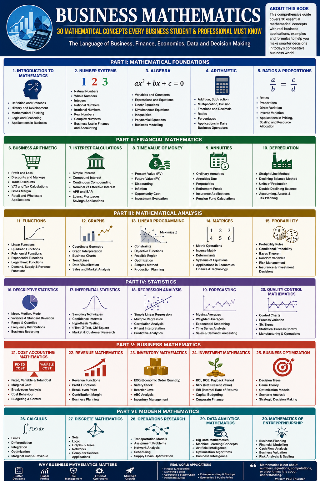
30 Essential Categories of Business Mathematics — Concepts, Formulas & Applied Business Practice
Contents
- Introduction
- 1. Foundations of Business Mathematics
- 2. Percentages, Ratios & Proportional Reasoning
- 3. Linear Equations & Break-Even Analysis
- 4. Simple Interest
- 5. Compound Interest
- 6. Annuities & Time Value of Money
- 7. Present Value & Net Present Value (NPV)
- 8. Internal Rate of Return (IRR) & Investment Appraisal
- 9. Depreciation Mathematics
- 10. Markup, Margin, Discount & Pricing Mathematics
- 11. Payroll, Commission & Wage Mathematics
- 12. Taxation Mathematics
- 13. Cost-Volume-Profit (CVP) Analysis
- 14. Financial Ratio Analysis
- 15. Descriptive Statistics for Business
- 16. Probability & Business Risk
- 17. Inferential Statistics & Hypothesis Testing
- 18. Regression Analysis & Forecasting
- 19. Index Numbers & Inflation Adjustment
- 20. Matrix Algebra in Business
- 21. Linear Programming & Optimization
- 22. Differential Calculus: Marginal Analysis
- 23. Integral Calculus in Business
- 24. Exponential & Logarithmic Growth Models
- 25. Bond Valuation Mathematics
- 26. Stock & Equity Valuation Mathematics
- 27. Foreign Exchange & International Trade Mathematics
- 28. Inventory Management Mathematics (EOQ)
- 29. Queuing Theory & Operations Research
- 30. Set Theory, Logic & Decision Trees in Business
- Closing Note
Introduction
This volume presents 30 categories of mathematics with a deliberate emphasis on business mathematics — the applied quantitative discipline underlying pricing, financing, forecasting, operations, and investment decisions across every industry.
Each category follows a consistent structure: a concise overview, the key formulas required, a fully worked numerical example, and the category’s real-world business application — designed to work equally well as a first introduction or a quick-reference manual.
1.Foundations of Business Mathematics
Business mathematics is the applied branch of mathematics used to model, measure, and optimise commercial decisions. It draws on arithmetic, algebra, statistics, and calculus, but reframes every operation around a business question: what does this number cost, earn, or risk. Mastery of the foundations below underpins every other category in this series.
Key Formulas
Order of operations: Brackets → Exponents → Multiplication/Division → Addition/Subtraction (BEMDAS)Percentage change = (New Value − Old Value) / Old Value × 100Unit conversion: Value in Unit B = Value in Unit A × Conversion Factor
Worked Example
Problem: A firm’s monthly revenue rises from R480,000 to R552,000.
Solution: Percentage change = (552,000 − 480,000) / 480,000 × 100 = 15%.
Business Application: Every dashboard, invoice, and budget a manager reads reduces to these foundational operations; errors here compound through every downstream calculation in finance, procurement, and reporting. Copy Section
2.Percentages, Ratios & Proportional Reasoning
Percentages and ratios translate absolute figures into comparable, decision-ready information. They allow a manager to compare a spaza shop’s margin with a JSE-listed retailer’s margin on equal footing, regardless of scale.
Key Formulas
Percentage of a value = (Part / Whole) × 100Ratio a:b simplification = a/GCD(a,b) : b/GCD(a,b)Direct proportion: y = kx | Inverse proportion: y = k/x
Worked Example
Problem: A company’s current assets are R2,400,000 and current liabilities R1,200,000.
Solution: Current ratio = 2,400,000 : 1,200,000 = 2:1, meaning the firm holds R2 of current assets per R1 of current liabilities.
Business Application: Working-capital ratios, gross-margin percentages, and debt-to-equity ratios are the daily vocabulary of financial managers, lenders, and investors. Copy Section
3.Linear Equations & Break-Even Analysis
Linear relationships model constant rates of change — a fixed cost structure plus a variable cost per unit. Break-even analysis finds the exact sales volume at which total revenue equals total cost.
Key Formulas
Total Cost (TC) = Fixed Costs (FC) + (Variable Cost per Unit × Quantity)Total Revenue (TR) = Price per Unit × QuantityBreak-even quantity (units) = FC / (Price − Variable Cost per Unit)
Worked Example
Problem: Fixed costs are R150,000; price per unit R250; variable cost per unit R150.
Solution: Break-even = 150,000 / (250 − 150) = 1,500 units, generating R375,000 in revenue at that point.
Business Application: Start-ups and product managers use break-even analysis before launch to decide whether projected market demand can realistically cover fixed overheads. Copy Section
4.Simple Interest
Simple interest grows a principal amount by a constant amount each period, calculated only on the original sum. It underlies short-term loans, trade credit terms, and some fixed-term promissory notes.
Key Formulas
I = P × r × tTotal Amount, A = P(1 + rt)Where P = principal, r = annual interest rate (decimal), t = time in years
Worked Example
Problem: R80,000 is borrowed at 9% simple interest for 8 months.
Solution: I = 80,000 × 0.09 × (8/12) = R4,800. Total repayment = R84,800.
Business Application: Trade financiers and short-term lenders use simple interest to keep repayment schedules transparent and easy for SME borrowers to verify manually. Copy Section
5.Compound Interest
Compound interest calculates interest on both the principal and previously accumulated interest, producing exponential rather than linear growth. It is the mathematical engine behind long-term savings, mortgages, and most modern lending.
Key Formulas
A = P(1 + r/n)^(nt)Effective annual rate (EAR) = (1 + r/n)^n − 1Continuous compounding: A = Pe^(rt)
Worked Example
Problem: R100,000 invested at 8% p.a., compounded monthly for 5 years.
Solution: A = 100,000(1 + 0.08/12)^(12×5) ≈ R149,024, versus R140,000 under simple interest — a R9,024 compounding premium.
Business Application: Retirement funds, unit trusts, and corporate bonds are priced and projected using compound interest; understanding compounding frequency materially changes reported returns. Copy Section
6.Annuities & Time Value of Money
An annuity is a series of equal payments made at regular intervals. Time value of money (TVM) formalises the principle that a rand today is worth more than a rand in the future, because today’s rand can be invested.
Key Formulas
Future Value of an Ordinary Annuity: FV = PMT × [((1+r)^n − 1) / r]Present Value of an Ordinary Annuity: PV = PMT × [(1 − (1+r)^-n) / r]Loan instalment: PMT = PV × r / (1 − (1+r)^-n)
Worked Example
Problem: A firm saves R20,000 per month for 3 years in an account earning 6% p.a. (0.5% monthly).
Solution: FV = 20,000 × [((1.005)^36 − 1)/0.005] ≈ R788,220.
Business Application: Pension contributions, sinking funds, equipment lease payments, and vehicle finance instalments are all annuity-based calculations. Copy Section
7.Present Value & Net Present Value (NPV)
Present value discounts a future cash flow back to today’s terms using an appropriate discount rate. NPV extends this to an entire investment’s cash-flow stream, netting the initial outlay against the sum of discounted returns.
Key Formulas
PV = FV / (1 + r)^nNPV = Σ [CFt / (1 + r)^t] − Initial InvestmentDecision rule: accept if NPV > 0
Worked Example
Problem: A project costs R500,000 and returns R200,000 per year for 3 years; discount rate 10%.
Solution: PV of cash flows ≈ 181,818 + 165,289 + 150,263 = R497,370. NPV = 497,370 − 500,000 = −R2,630 → marginally reject.
Business Application: NPV is the primary capital-budgeting tool for boards deciding between competing projects, acquisitions, or expansion options. Copy Section
8.Internal Rate of Return (IRR) & Investment Appraisal
IRR is the discount rate at which a project’s NPV equals exactly zero — the effective annualised return the project itself generates. It is typically solved iteratively or via financial software rather than algebraically.
Key Formulas
0 = Σ [CFt / (1 + IRR)^t] − Initial InvestmentPayback Period = Initial Investment / Annual Cash Inflow (even cash flows)Profitability Index = PV of Future Cash Flows / Initial Investment
Worked Example
Problem: A machine costs R1,000,000 and returns R300,000 per year for 5 years.
Solution: Trial-and-error/interpolation places IRR at approximately 15.2%, above the firm’s 12% hurdle rate, so the project is accepted.
Business Application: Investment committees compare IRR against a hurdle rate (cost of capital) to rank capital projects competing for the same limited budget. Copy Section
9.Depreciation Mathematics
Depreciation allocates the cost of a tangible asset over its useful life, reflecting wear, obsolescence, or usage. The method chosen affects reported profit, tax liability, and balance-sheet asset values.
Key Formulas
Straight-line: Annual Depreciation = (Cost − Residual Value) / Useful LifeReducing balance: Depreciation = Book Value × Depreciation RateUnits of production: Depreciation = (Cost − Residual Value) × (Units Produced / Total Estimated Units)
Worked Example
Problem: A delivery truck costs R450,000, residual value R50,000, useful life 8 years.
Solution: Straight-line depreciation = (450,000 − 50,000)/8 = R50,000 per year.
Business Application: Fleet-owning and manufacturing businesses select depreciation methods to match tax strategy and to present asset values accurately to lenders and auditors. Copy Section
10.Markup, Margin, Discount & Pricing Mathematics
Pricing mathematics converts cost data into a selling price using either markup (percentage of cost) or margin (percentage of selling price) — two related but frequently confused concepts.
Key Formulas
Markup % = (Selling Price − Cost) / Cost × 100Margin % = (Selling Price − Cost) / Selling Price × 100Discounted Price = List Price × (1 − Discount Rate)
Worked Example
Problem: A retailer buys stock at R400 and sells at R600.
Solution: Markup = (600−400)/400 × 100 = 50%. Margin = (600−400)/600 × 100 = 33.3% — the same transaction, two different figures.
Business Application: Confusing markup with margin is one of the most common pricing errors in retail and e-commerce, directly distorting profitability forecasts. Copy Section
11.Payroll, Commission & Wage Mathematics
Payroll mathematics computes gross pay, statutory deductions, and net pay across hourly, salaried, and commission-based structures, forming the operational core of human-resources and finance functions.
Key Formulas
Gross Pay (hourly) = Hours Worked × Rate + Overtime Hours × Rate × 1.5Commission Earned = Sales Value × Commission RateNet Pay = Gross Pay − (Tax + UIF + Other Deductions)
Worked Example
Problem: A sales rep earns a R8,000 base plus 6% commission on R320,000 of sales.
Solution: Commission = 320,000 × 0.06 = R19,200. Gross pay = 8,000 + 19,200 = R27,200.
Business Application: Accurate commission mathematics directly affects sales-force motivation and trust; payroll errors are among the fastest ways a business erodes staff confidence. Copy Section
12.Taxation Mathematics
Taxation mathematics applies progressive or flat rate structures to income, turnover, or transactions to determine liability owed to revenue authorities, a mandatory calculation for every registered entity.
Key Formulas
Progressive tax: Tax = Σ (Bracket Amount × Bracket Rate)VAT-exclusive price = VAT-inclusive price / (1 + VAT rate)Effective tax rate = Total Tax Paid / Taxable Income × 100
Worked Example
Problem: A product sells for R1,150 VAT-inclusive at a 15% VAT rate.
Solution: VAT-exclusive price = 1,150 / 1.15 = R1,000; VAT portion = R150.
Business Application: Every invoice a South African business issues embeds this VAT calculation; miscalculating it creates compliance risk with SARS and cash-flow discrepancies. Copy Section
13.Cost-Volume-Profit (CVP) Analysis
CVP analysis extends break-even mathematics to examine how changes in costs, price, and volume interact to affect operating profit, supporting pricing, budgeting, and product-mix decisions.
Key Formulas
Contribution Margin per Unit = Selling Price − Variable Cost per UnitContribution Margin Ratio = Contribution Margin per Unit / Selling PriceTarget Profit Units = (Fixed Costs + Target Profit) / Contribution Margin per Unit
Worked Example
Problem: Contribution margin per unit is R80; fixed costs R400,000; target profit R160,000.
Solution: Target units = (400,000 + 160,000) / 80 = 7,000 units required.
Business Application: Finance teams use CVP modelling before setting annual sales targets, ensuring targets are mathematically consistent with cost structure and profit goals. Copy Section
14.Financial Ratio Analysis
Financial ratios compress complex financial statements into standardised indicators of liquidity, profitability, efficiency, and solvency, enabling comparison across time periods and between competitors.
Key Formulas
Gross Profit Margin = Gross Profit / Revenue × 100Return on Equity (ROE) = Net Income / Shareholders' Equity × 100Debt-to-Equity = Total Liabilities / Shareholders' Equity
Worked Example
Problem: Net income is R3,600,000 and shareholders’ equity R18,000,000.
Solution: ROE = 3,600,000 / 18,000,000 × 100 = 20%.
Business Application: Investors and credit committees use ratio analysis as the first screening step before deeper due diligence on any prospective investment or loan. Copy Section
15.Descriptive Statistics for Business
Descriptive statistics summarise raw business data — sales figures, customer ages, transaction sizes — into central tendency and dispersion measures that reveal patterns invisible in the raw dataset.
Key Formulas
Mean = Σx / nStandard Deviation, σ = √[Σ(x − mean)² / n]Coefficient of Variation = (σ / mean) × 100
Worked Example
Problem: Weekly sales (R’000): 120, 135, 128, 150, 142.
Solution: Mean = 135; Standard deviation ≈ 10.6; Coefficient of variation ≈ 7.9%, indicating relatively stable weekly sales.
Business Application: Standard deviation of sales or demand feeds directly into inventory buffer stock and staffing-level decisions. Copy Section
16.Probability & Business Risk
Probability quantifies uncertainty, giving managers a structured way to weigh the likelihood of outcomes such as loan default, project delay, or supply disruption.
Key Formulas
P(A) = Favourable Outcomes / Total Possible OutcomesP(A and B) = P(A) × P(B) for independent eventsExpected Value = Σ [Outcome Value × Probability of Outcome]
Worked Example
Problem: A project has a 70% chance of R500,000 profit and 30% chance of a R200,000 loss.
Solution: Expected value = (0.7 × 500,000) + (0.3 × −200,000) = 350,000 − 60,000 = R290,000.
Business Application: Insurance pricing, credit-risk scoring, and portfolio diversification all rely on expected-value and probability calculations. Copy Section
17.Inferential Statistics & Hypothesis Testing
Inferential statistics use a sample to draw conclusions about a wider population, allowing a business to test claims — such as whether a new marketing campaign genuinely increased conversion rates — with quantified confidence.
Key Formulas
z-score = (x − μ) / σConfidence Interval = Sample Mean ± (z × Standard Error)t-test statistic = (Mean1 − Mean2) / Standard Error of Difference
Worked Example
Problem: A sample of 100 customers has a mean spend of R450 with a standard deviation of R60.
Solution: Standard error = 60/√100 = 6. 95% confidence interval ≈ 450 ± (1.96×6) = R438.24 to R461.76.
Business Application: A/B testing of pricing, advertising, and website design in e-commerce depends entirely on hypothesis-testing mathematics to separate genuine effect from random noise. Copy Section
18.Regression Analysis & Forecasting
Regression models the relationship between a dependent variable (such as sales) and one or more independent variables (such as advertising spend), enabling forecasting and scenario planning.
Key Formulas
Simple linear regression: y = a + bxSlope, b = [nΣxy − ΣxΣy] / [nΣx² − (Σx)²]Coefficient of determination, R² = explained variation / total variation
Worked Example
Problem: Regression of monthly ad spend on sales yields y = 50,000 + 4.2x.
Solution: At an ad spend of R30,000, forecast sales = 50,000 + (4.2 × 30,000) = R176,000.
Business Application: Demand forecasting, revenue budgeting, and marketing-mix modelling in Amazon and Takealot-style e-commerce operations lean on regression to plan inventory and cash flow. Copy Section
19.Index Numbers & Inflation Adjustment
Index numbers measure relative change in a variable — prices, output, wages — against a fixed base period, the mathematical foundation of inflation reporting and real (inflation-adjusted) value comparisons.
Key Formulas
Price Index = (Current Period Price / Base Period Price) × 100Real Value = Nominal Value / (Price Index / 100)Inflation Rate = (CPI_current − CPI_previous) / CPI_previous × 100
Worked Example
Problem: A salary of R30,000 in 2020 (CPI 100) should be compared to 2026 (CPI 138).
Solution: Real 2026-equivalent salary = 30,000 × 1.38 = R41,400 needed just to maintain 2020 purchasing power.
Business Application: Salary negotiations, long-term contract escalation clauses, and multi-year budget comparisons all require index-based inflation adjustment to remain meaningful. Copy Section
20.Matrix Algebra in Business
Matrices organise multi-dimensional business data — such as production quantities across several products and factories — into a structure that supports efficient combined calculation.
Key Formulas
Matrix multiplication: (AB)ij = Σk Aik × BkjIdentity Matrix, I: AI = IA = AInverse Matrix: A × A⁻¹ = I (used to solve simultaneous equations)
Worked Example
Problem: Two factories produce Product X and Y; a cost matrix and a quantity matrix are multiplied to get total cost per factory.
Solution: Matrix multiplication aggregates unit costs across products in a single operation instead of multiple separate sums, reducing computation error at scale.
Business Application: Enterprise resource planning (ERP) systems and multi-product cost allocation models are built on matrix operations behind the scenes. Copy Section
21.Linear Programming & Optimization
Linear programming finds the best outcome — maximum profit or minimum cost — subject to a system of linear constraints, such as limited labour hours, raw materials, or shelf space.
Key Formulas
Objective function: Maximise Z = c1x1 + c2x2Subject to constraints: a1x1 + a2x2 ≤ b (resource limits)Non-negativity constraint: x1, x2 ≥ 0
Worked Example
Problem: A factory maximises profit Z = 40x + 30y subject to 2x + y ≤ 100 (labour) and x + 3y ≤ 90 (material).
Solution: Solving at the constraint intersection gives x = 42, y = 16, yielding Z ≈ R2,160, the optimal product mix.
Business Application: Production scheduling, delivery-route planning, and shelf-space allocation in retail and logistics are classic linear-programming applications. Copy Section
22.Differential Calculus: Marginal Analysis
Differential calculus measures instantaneous rates of change. In business, the derivative of a cost or revenue function gives marginal cost or marginal revenue — the cost or revenue of producing one additional unit.
Key Formulas
Marginal Cost = dTC/dQMarginal Revenue = dTR/dQProfit-maximising condition: Marginal Revenue = Marginal Cost
Worked Example
Problem: Total Revenue TR = 100Q − 2Q². Total Cost TC = 20Q + 500.
Solution: MR = 100 − 4Q; MC = 20. Setting MR = MC: 100 − 4Q = 20 → Q = 20 units maximises profit.
Business Application: Pricing teams use marginal analysis to decide whether producing or selling one more unit still adds more revenue than it costs. Copy Section
23.Integral Calculus in Business
Integral calculus accumulates rates of change into totals — such as total cost from marginal cost, or the area representing consumer and producer surplus in a market.
Key Formulas
Total Cost from Marginal Cost: TC = ∫ MC dQ + Fixed CostsConsumer Surplus = ∫₀^Q [Demand Price − Market Price] dQAccumulated value from a continuous cash-flow rate: V = ∫ f(t) dt
Worked Example
Problem: Marginal cost MC = 10 + 0.5Q; fixed costs R2,000.
Solution: TC = ∫(10 + 0.5Q)dQ + 2,000 = 10Q + 0.25Q² + 2,000.
Business Application: Consumer and producer surplus calculations inform competition-policy analysis and welfare assessments of pricing strategies. Copy Section
24.Exponential & Logarithmic Growth Models
Exponential functions model quantities that grow proportionally to their current size — compound interest, market penetration, and viral customer acquisition — while logarithms invert exponential relationships to solve for time or rate.
Key Formulas
Exponential growth: N(t) = N0 × e^(kt)Doubling time = ln(2) / kSolving for time in compound interest: t = ln(A/P) / [n × ln(1 + r/n)]
Worked Example
Problem: How long until R50,000 grows to R100,000 at 9% compounded annually?
Solution: t = ln(2) / ln(1.09) ≈ 8.04 years.
Business Application: Subscription businesses use exponential models to project user-base growth and to estimate the time needed to reach a target customer count. Copy Section
25.Bond Valuation Mathematics
Bond valuation discounts a bond’s promised coupon payments and face-value repayment to present value using the market’s required yield, determining the fair price an investor should pay.
Key Formulas
Bond Price = Σ [Coupon / (1+y)^t] + Face Value / (1+y)^nCurrent Yield = Annual Coupon / Current Market PriceYield to Maturity (YTM): the rate y solving the bond price equation exactly
Worked Example
Problem: A 3-year bond, face value R1,000, 8% annual coupon, required yield 10%.
Solution: Price ≈ 80/1.10 + 80/1.10² + 1,080/1.10³ ≈ 72.73 + 66.12 + 811.42 = R950.27, trading at a discount because the coupon is below the required yield.
Business Application: Corporate treasuries and fixed-income fund managers price bonds and estimate portfolio value shifts as interest rates move using this exact framework. Copy Section
26.Stock & Equity Valuation Mathematics
Equity valuation estimates a share’s intrinsic worth from expected future dividends or cash flows, providing a mathematical benchmark against the current market price.
Key Formulas
Gordon Growth (Dividend Discount) Model: P0 = D1 / (r − g)Price-Earnings Ratio = Market Price per Share / Earnings per ShareDividend Yield = Annual Dividend per Share / Share Price × 100
Worked Example
Problem: A share is expected to pay a R5 dividend next year, growing at 4% annually; required return 12%.
Solution: P0 = 5 / (0.12 − 0.04) = R62.50 — compared against the current market price to judge over- or under-valuation.
Business Application: Portfolio managers running the international, JSE, and Dubai Stake portfolios use these models alongside market ratios to assess whether a stock is attractively priced. Copy Section
27.Foreign Exchange & International Trade Mathematics
Foreign exchange mathematics converts values between currencies and adjusts for the cost of hedging or delayed settlement, essential wherever a business imports, exports, or invests across borders.
Key Formulas
Direct conversion: Amount in Currency B = Amount in Currency A × Spot RateCross rate: Rate(A/C) = Rate(A/B) × Rate(B/C)Forward rate ≈ Spot Rate × [(1 + Domestic Interest) / (1 + Foreign Interest)]
Worked Example
Problem: R1,000,000 is converted to USD at a spot rate of R18.50/USD.
Solution: USD amount = 1,000,000 / 18.50 = USD 54,054.05.
Business Application: Import/export businesses and multi-currency investment portfolios must apply spot, cross, and forward-rate mathematics to manage currency exposure and settlement timing. Copy Section
28.Inventory Management Mathematics (EOQ)
Economic Order Quantity (EOQ) mathematics balances the cost of ordering stock too frequently against the cost of holding excess inventory, identifying the order size that minimises total inventory cost.
Key Formulas
EOQ = √[(2 × Annual Demand × Ordering Cost) / Holding Cost per Unit]Total Inventory Cost = (D/Q)×Ordering Cost + (Q/2)×Holding CostReorder Point = Average Daily Usage × Lead Time in Days
Worked Example
Problem: Annual demand 12,000 units; ordering cost R250 per order; holding cost R6 per unit per year.
Solution: EOQ = √[(2×12,000×250)/6] = √1,000,000 = 1,000 units per order.
Business Application: E-commerce and retail operations use EOQ mathematics to set purchase-order sizes for Amazon and Takealot fulfilment stock, minimising warehousing and stock-out costs simultaneously. Copy Section
29.Queuing Theory & Operations Research
Queuing theory mathematically models waiting lines — customers at a till, calls at a support centre — to determine optimal staffing and service-capacity levels against a target wait time.
Key Formulas
Traffic Intensity, ρ = λ / μ (arrival rate ÷ service rate)Average number in system (M/M/1 queue): L = ρ / (1 − ρ)Average waiting time in queue: Wq = ρ² / [λ(1 − ρ)]
Worked Example
Problem: Customers arrive at 8 per hour (λ); a till serves 10 per hour (μ).
Solution: ρ = 8/10 = 0.8. Average customers in system L = 0.8/(1−0.8) = 4 customers, signalling the till is close to overload.
Business Application: Call-centre staffing and checkout-counter planning use queuing mathematics to balance customer wait time against staffing cost. Copy Section
30.Set Theory, Logic & Decision Trees in Business
Set theory and formal logic structure business rules and categorisation (customer segments, product overlaps), while decision trees apply probability across sequential business choices to identify the highest expected-value path.
Key Formulas
Union: A ∪ B; Intersection: A ∩ B; Complement: A′Inclusion-Exclusion: |A ∪ B| = |A| + |B| − |A ∩ B|Decision tree expected value at each node = Σ (Branch Probability × Branch Payoff)
Worked Example
Problem: Of 500 customers, 300 bought Product A, 250 bought Product B, and 120 bought both.
Solution: Customers who bought at least one product = 300 + 250 − 120 = 430, using the inclusion-exclusion principle directly.
Business Application: Customer-segmentation overlap analysis and multi-stage strategic decisions (enter a new market vs. not, under uncertain demand) are formalised using set theory and decision-tree expected-value mathematics. Copy Section
Closing Note
The thirty categories in this volume represent the working toolkit most consistently applied across finance, operations, statistics, and strategy functions in a modern business. Fluency across all thirty — rather than depth in only one or two — is what distinguishes a manager who can converse credibly with accountants, actuaries, economists, and data scientists alike.






Be First to Comment